Top 10 Excel Formulas Interview Questions and Answers

Following are the Most Frequently Asked Excel Formulas in an interview

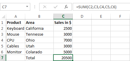
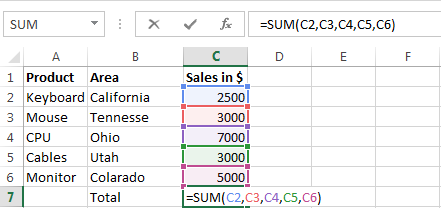
1) SUM formula: =SUM (C2,C3,C4,C5)

In excel, SUM formula is used to calculate the total number.  For instance here we had calculated the total number of computer items sold across different region in U.S.A by using formula =SUM (C2,C3,C4,C5) at the end you get the total $ 20, 500, as shown in next formula. In formula, inside bracket you have to mention the column or row number which you want to add.

2) Average Formula: = Average (C2,C3,C4,C5)

In excel, the average formula, is used to retrieve the average for any number. Like we have calculated the average sales of computer merchandise across U.S.A. The first screen shot highlights the formula, i.e., = Average (C2,C3,C4,C5) that we have applied for our data.

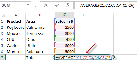
The below screen shot shows the average amount that we retained after applying the formula.

3) SumIF formula = SUMIF (A2:A7,“Items wanted”, D2:D7)

The SumIF gives the total number of any items for selected ranges. For instance here we want to calculate only the total sales amount for software items, to do that we will apply the formula as =SUMIF (A2:A7, “software”, D2:D7).  Here A2 and A7 defines the range for software and same way we can find sales amount for hardware. (A2:A7, “software”, D2:D7).

 

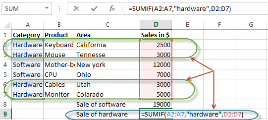
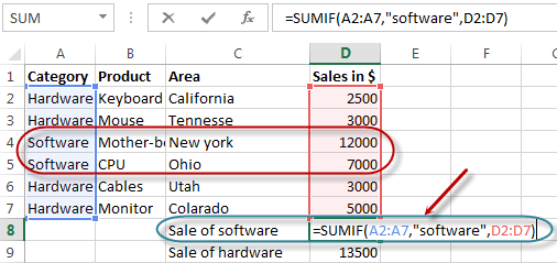
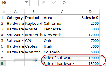
Below screen-shot show the total sale amount of hard-ware and soft-ware in the table.

4) COUNTIF Formula: COUNTIF(D2:D7, “Function”)

COUNTIF function offers wide application; you can apply the formula according. Here we have taken a simple example of COUNTIF function, where our motive is to find the total number of cells whose value is greater than $3000. In order to know that we will apply the formula =COUNTIF(D2:D7,”3000”).

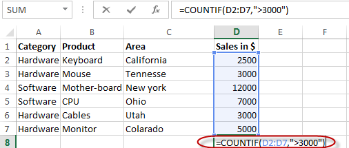
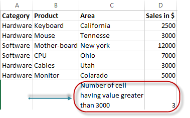
Below screen shot shows the total number of cells that has value greater than 3000.

5) Concatenate Function: =CONCATENATE(C4,Text, D4, Text,…)

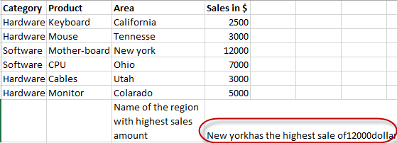
Concatenate function is used in excel to connect different segment or text to display as a single sentence. For example, here we want to display text as “NewYork has the highest sale of 12000 dollars”, for that we will use the formula =CONCATENATE(C4,”has the highest sale of”,D4,dollar”).

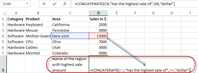
When you execute the formula and display the text as show in below screen-shot

6) Int Formula: int (this number)

Int formula is used to remove integer from the number like we have demonstrated over here in below example.

7) MAX Formula: =Max(D2:D7)

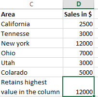
This excel formula will retain the cells that have the highest value in the column, for example, here we want to know the highest value for computer items, and it retains the value $12000. Likewise, you can execute same formula to get a minimum value, in the formula you have to replace Max with Min.

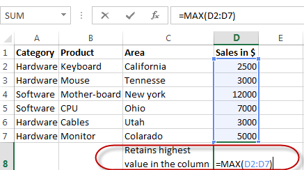
Below, screen shot shows the highest value in the column.

8) Factorial Formula= FACT(number)

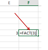
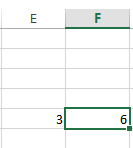
Factorial formula will return the factorial of the number. To know the factorial number for 3, we use this formula.  You can use this formula to know the probability for any number, here we will have factor 3=3x2x1.

 

9) VLookup Formula = Vlookup(value, range, and get me value in the column, is my list sorted)

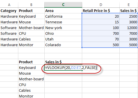
VLookup formula is used when you know anyone detail of any object or person and, you retain other formation based on that detail. For example here we have an example of the keyboard, where you know the retail price of the keyboard but you don’t know how much total sale it made in California by selling keyboard. To know that you will use =Vlookup(20,D2:D7,2,False).  This formula will give you the total sale amount based on the retail price.  While applying this formula you have ensure that whatever you are placing as ref, must be unique, for example you are looking for any particular employee with its ID number it should not be allotted to others otherwise it will show an error.

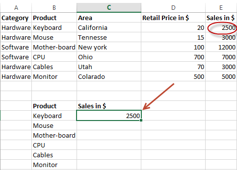
When formula is executed, the total sale amount shown is $2500

10) IF function formula: IF (E2>2000, correct/Incorrect)

Here we have used IF function; this function is used when you want to refer whether the following condition met is correct or incorrect.  Here we have used “good” as any sales made greater than 2000 should be remarked as good. Likewise, you can set this as “bad”, “correct” or “incorrect”.

Below table shows when we applied our formula it highlighted cell as “good”.

Which other formulas were asked to you in an interview? Let us know in comments below –